All is loss
You might have heard, that most supervised Machine Learning methods boil down to minimizing a loss function over a set of parameters. I for myself was somewhat aware of this for a long time, but it was not until recently that I realized how powerfull this observation really is.
-
Generality. Literally the same ideas apply to linear regressions, also used for training neural networks and SVMs.
-
Effectivity. The above minimization can be performed with general numeric methods. This works in practice. While there shortcuts for some cases in most cases this the only thing you can do.
-
Geometry. Being a trained as an algebraic geometer, I enjoy geometric approaches to problems. We will take a geometric view in this article, and draw some pretty pictures of paramters and model values.
In this blog post we will first introduce the general machinery of loss minimization, and then visit a number of different machine learning models in this context.
The General Loss Function
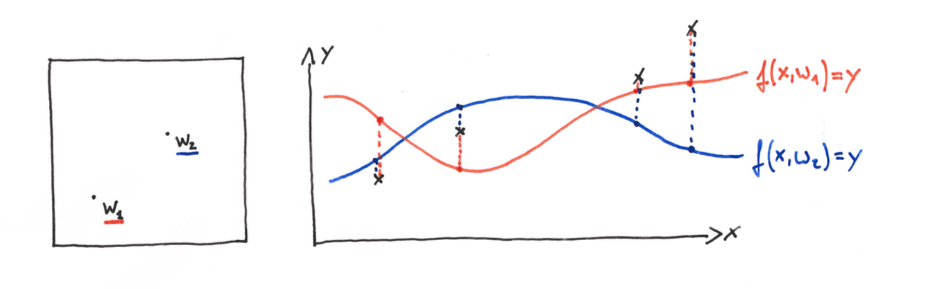
In a supervised learning setup, we commonly consider a free variable $x$ and a target variable $y$. (We are purposefully vague about the nature of $x$ and $y$ here, they can take one-dimensional, vector, or discrete values). For a given $x$ we want to determine the likely value of $y$. To do so, we introduce a modeling step. We consider a family of possible relations $f:x \mapsto y$ that are parametrized by a parameter $w$:
The question becomes, which model parameter $w$, will give us a good model?
In order to settle for some parameter $w$, we need some evidence encoded in a training dataset $D=(x_i,y_i)_i, i=1,\dots,N$. This gives us some examples of the relation $x \mapsto y$ that we seek to generalize. The training objective is now to find a parameter $w=\hat{w}$, so that a
for $x_i,y_i$ in the training dataset $D$.
A common mathematical measure of “closeness” is the absolute distance $|a-b|$ in case that $y$ takes value in $\mathbb{R}$. More generally, we can consider a distance function $d(a,b)$ with $d(a,b) \geq 0$ and $d(a,a)=0$ to quantify the distance. Given such a distance $d$, we can then define a loss function as
Note that the loss function, only depends on the model parameter $w$, and on the training dataset. There is no dependency on $x$ and $y$ anymore.
The task of fitting the model to the training data can now be formulated as a minimization problem. Find a parameter $\hat{w}$, so that $Loss_D(w)$ is minimal:
Once we have found $\hat{w}$, we can estimate the target variable $y$ from a given $x$:
How good this model turns out to preform in practice depends heavily on the training data and the family of models we have been taking into consideration. However, the training procedure is always the same.
Effectivity: A implementation in Python
To implement a supervised machine learning model in python, one only needs to implement two functions:
def f(x,w):    # model function, e.g. w[0] + w[1]*x[0]
def dist(a,b): # distance function, e.g (a-b)^2
The rest is general machinery:
def Loss(w,D):
    loss = 0
    for i in range(len(D['x'])):
        x = D['x'][i]
        y = D['y'][i]
        loss += dist(f(x,w),y)
    return loss

from scipy.optimize import minimize
w0 = [...]                            # initiailization parameter
M = minimize(lambda w: Loss(w,D), w0) # Numeric minimization
print(M.x)                            # print results
Strikingly simple! No?
Granted, this will not give the most effective minimizer in most cases, but as we will see this already works quite well. State of the art methods, only differ in the minimization method that is used. In particular information about gradient and Hessian matrix of the loss function might be available, and can be exploited.
An example Dataset
To make things fun an concrete we consider a (totally made up) dataset for some machine parts.
| Current | Voltage | Vibration | Error-rate | Faulty | |
|---|---|---|---|---|---|
| 0.61 | 9.9 | 24.7 | 0.02 | 0 | |
| 0.53 | 14.9 | 26.2 | 0.01 | 0 | |
| 0.45 | 15.9 | 22.7 | 0.01 | 0 | |
| 0.32 | 15.8 | 234.1 | 6.51 | 1 | |
| 0.38 | 11.8 | 254.3 | 6.24 | 1 | |
| … |
Each part comes with three sensor readings “current”, “voltage” and “vibration” that act as free variables. The remaining two variables “error-rate” and “faulty” are the target variables we seek to predict.
Method 0: Manual Examination
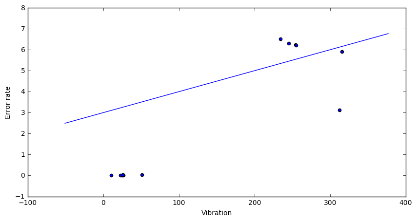
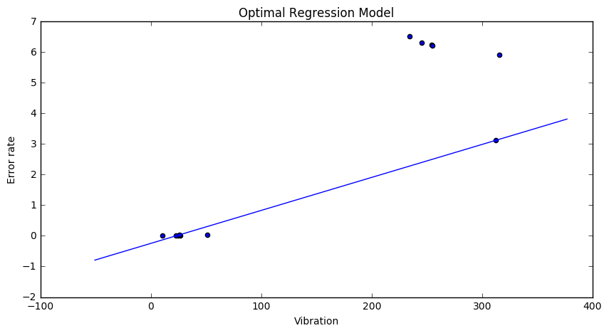
Looking at the data it’s pretty clear that error-rate faulty can be determined from the vibration reading. The first two variables are uncorrelated. Here is a scatterplot that visualizes the relation between “vibration” and “error-rate”.

If the vibration parameter goes above ~100 we expect a high error rate and a faulty part. This is what the learning methods below should show as well.
Method 1: Linear Regression
The first model we consider is the linear regression model. To apply the above procedure, we must only specify a model function $f(x,w)$ and a distance $d$. For linear regressions we put:
Here N would be the number of free variables (3 in our case) and $x_1,\dots,x_N$ the values of a single row of data in the table. E.g. $(x_1,x_2,x_3)=(0.61,9.9,24.7)$.
To make things even more simple, we consider the one-dimensional case here (N=1) and consider only the “vibration” variable.
As distance function we will take the squared difference $d(a,b) = (a-b)^2$, so
With the dataset at hand we can now make this concrete. Let’s choose some arbitrary parameters $(w_0,w_1)=(-3,1)$ then we compute:
The corresponding model looks clearly terrible:
We can visualize the loss function over a whole range of parameters using a heatmap:
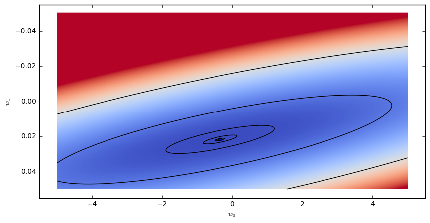
Each point in the plane, corresponds to choice of parameters $w_0,w_1$. The color indicates the value of the loss function $Loss_D(w_0,w_1)$. Dark/blue colors correspond to low values, red colors correspond to large values.
The minimal loss is realized by the choice of parameters:
The corresponding model looks already much better:

Method 2: Variation on Linear Regression
With the general machinery in place, we can play around with the model and distance function to arrive at different regression model. For example we could change the distance function, to be the absolute value and not the square difference. Also we might, just for fun, cap the maximal loss-contribution of a single sample at one, so:
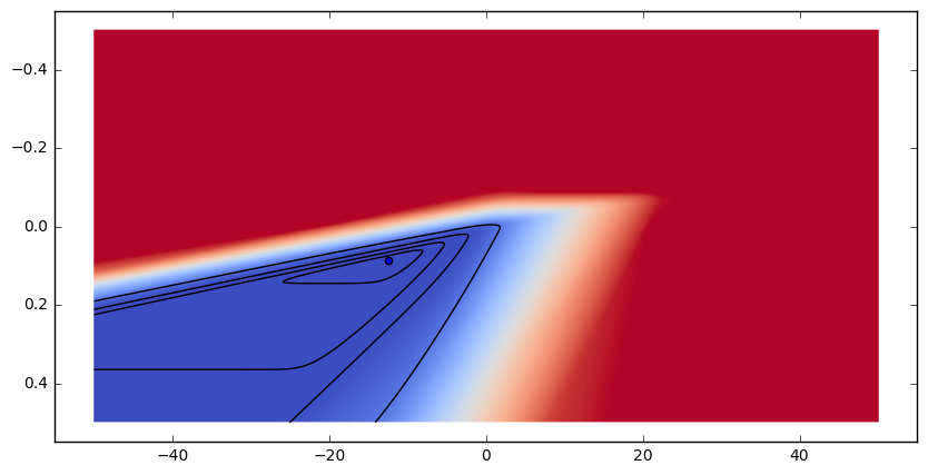
The model function remains the same as for linear regression above. The resulting loss function looks as follows:
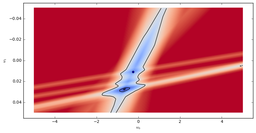
This time python’s minimizer get’s stuck in a local minimum $(w_0,w_1)=(-0.24, 0.01)$ (represented by a dot in the above figure) and the fitted model looks less then ideal:
Apparently this very distance function is not very suited for practical applications.
Method 3: Logistic Regression
The logistic regression model predicts a binary variable $y=0,1$ from a continuous input $x$. It uses the following model function:
where $\sigma(x) = 1/(1+\exp(-x))$ is the sigmoid function. The distance function is given by:
These choices may seem a bit unnatural. Instead of motivating them here, we just note that $\sigma(x)$ is an “S”-shaped function with values in $[0,1]$, and that d(a,b) is a distance measure that makes complete mispredictions very expensive ($d(1,0) = \infty$).
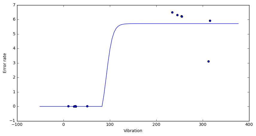
Fitting a logistic regression model to the “vibration” and “error rate” examples looks as follows:

Note that there is a large sector of parameters, where the loss function is near constant (zero). It turns out that the loss function does not have a global minimum in this case. One can further decrease the loss by moving further “out” along this sector. At some point Python’s minimizer just stops to care and returns a value.
The resulting model looks like this:

We can enforce the existence of a minimum by adding a so called regularization term to the loss function, e.g.
This will penalize sharp ascends, and least to the following loss and model functions:
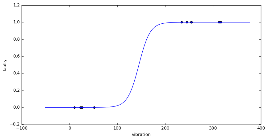
Ahh, that’s much better. There is a global unique minimum that the Python mimimizer had no trouble finding. Also the resulting model is less extreme than before. It looks well adapted to the training data, but not overfitted.
Method 4: Neural Nets
You might be shocked to hear that neural networks are just stacked logistic regressions. So the model looks like this
Since we want to apply this network to a regression problem, will chose a “ReLU” activation function as output transformation:
In this way we will have a chance to fit data that is not confined to the $[0,1]$ range. For the distance function we chose the squared difference:
Since the model has more than two parameters, we need to fix all but two of them before we can visualize the Loss function. The following images illustrates the Loss functions in the variables $w_0$,$w_3$, with $w_1=0.14,w_2-1.6$.
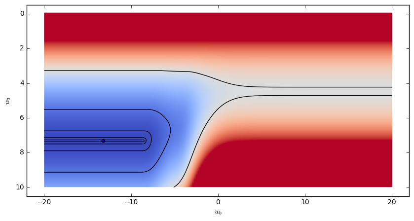
The resulting model looks like this:
Clearly visible are the ReLU cutoff just before x=100, and the scaled sigmoid function in the $x>100$ region. The resulting models is very sensitive to the chosen initial parameters for the minimization.
Conclusion
We have seen how the loss minimizations gives a general and effective framework to approach a number of different supervised learning methods. We only ended up treating one-dimensional examples, the general case is not conceptually more difficult, just harder to visualize.
One thing I took away while writing this is how the complexity of the distance and model function can affect the performance of the minimizer. It’s easy to end up with loss functions that have lot’s of local minima, and the fitted model is heavily dependent on the initial parameters. There is certainly an art in choosing those functions in such a way that the minimization can be performed effectively while making the model rich and robust enough for applications.
Epilogue
The jupyter notebooks used to generated the graphics are available here.
If you liked this post, you migh also find these visuaulzations of differet optimization algorithms by Alac Radford interesting.
This post drew some inspiration from a video lecture by Romeo Kienzler.
Thanks to Rene Pickhardt and Martin Thoma for their feedback on earlier versions of this article.